17  Combining Datasets

17.1 Introduction: Why Combine Datasets?

In real-world data analysis, information is rarely contained in a single dataset. You’ll often need to combine multiple datasets from different sources to get a complete picture. This process is fundamental to data analysis and goes by several names:

• Merging - joining datasets based on common keys
• Joining - combining datasets using indices
• Concatenating - stacking datasets vertically or horizontally

17.1.1 Common Scenarios Requiring Data Combination

1. Distributed Information

• Customer demographics in one table, purchase history in another
• Product details separate from sales transactions
• Survey responses split across multiple files

2. Data from Multiple Sources

• Internal company data + external market data
• Multiple databases (HR, Sales, Inventory)
• Different time periods stored in separate files

3. Analytical Requirements

• Enriching existing data with additional attributes
• Comparing data across different groups or time periods
• Building comprehensive datasets for machine learning

17.1.2 The Three Main Combination Methods

Pandas provides three powerful functions for combining datasets, each suited to different scenarios:

Method	Function	Use Case	Key Parameter
Merge	merge()	Combine datasets with common columns (like SQL JOIN)	on= (column name)
Join	join()	Combine datasets using their indices	lsuffix=, rsuffix=
Concatenate	concat()	Stack datasets vertically or horizontally	axis= (0 or 1)

In this chapter, we’ll explore each method with practical examples, understand when to use which approach, and learn how to handle common challenges like missing values and duplicate columns.

17.1.3 Setup: Loading Required Libraries

Let’s start by importing the necessary libraries and loading our example datasets.

import pandas as pd
import numpy as np
import matplotlib.pyplot as plt
import seaborn as sns

# Display settings for better output
pd.set_option('display.max_columns', None)
pd.set_option('display.width', None)

17.2 Method 1: Merging with merge()

The merge() function is pandas’ most versatile tool for combining datasets. It works similarly to SQL JOIN operations, combining DataFrames based on one or more common columns (called keys).

17.2.1 Basic Syntax

pd.merge(left_df, right_df, on='key_column', how='inner')

Or using the DataFrame method:

left_df.merge(right_df, on='key_column', how='inner')

Let’s see this in action!

17.2.2 Example Datasets: Lord of the Rings Fellowship

Throughout this chapter, we’ll use multiple datasets that contain complementary information, we’ll combine using different methods.

Let’s first load the primary dataset containing basic fellowship member information:

# Load the primary dataset
df_existing = pd.read_csv('./datasets/LOTR.csv')

print(f"Dataset shape: {df_existing.shape}")
print(f"Columns: {list(df_existing.columns)}\n")

df_existing.head()

Dataset shape: (4, 3)
Columns: ['FellowshipID', 'FirstName', 'Skills']

	FellowshipID	FirstName	Skills
0	1001	Frodo	Hiding
1	1002	Samwise	Gardening
2	1003	Gandalf	Spells
3	1004	Pippin	Fireworks

Now let’s load the external dataset containing additional information about the fellowship members:

# Load the external dataset
df_external = pd.read_csv("./datasets/LOTR 2.csv")

print(f"Dataset shape: {df_external.shape}")
print(f"Columns: {list(df_external.columns)}\n")

df_external.head()

Dataset shape: (5, 3)
Columns: ['FellowshipID', 'FirstName', 'Age']

	FellowshipID	FirstName	Age
0	1001	Frodo	50
1	1002	Samwise	39
2	1006	Legolas	2931
3	1007	Elrond	6520
4	1008	Barromir	51

Observation: Both datasets contain information about fellowship members, but they may have:

• Common columns that can serve as keys for merging (like FellowshipID or Name)
• Different sets of attributes that complement each other
• Potentially different numbers of rows (not all members may appear in both datasets)

Our goal is to combine these datasets to create a comprehensive view of the fellowship.

17.2.3 Example 1: Basic Merge with Automatic Key Detection

When both DataFrames have columns with the same name, merge() automatically uses them as keys:

# Merge using automatic key detection
df_merged = pd.merge(df_existing, df_external)

print(f"Original datasets: {df_existing.shape} + {df_external.shape}")
print(f"Merged dataset: {df_merged.shape}")
print(f"\nMerged columns: {list(df_merged.columns)}\n")

df_merged.head()

Original datasets: (4, 3) + (5, 3)
Merged dataset: (2, 4)

Merged columns: ['FellowshipID', 'FirstName', 'Skills', 'Age']

	FellowshipID	FirstName	Skills	Age
0	1001	Frodo	Hiding	50
1	1002	Samwise	Gardening	39

Alternative Syntax: You can also use the DataFrame method, which is more readable in method chains:

# Using DataFrame.merge() method (equivalent to above)
df_merged_method = df_existing.merge(df_external)

print(f"Results are identical: {df_merged.equals(df_merged_method)}")
print(f"Merged dataset shape: {df_merged_method.shape}\n")

df_merged_method.head()

Results are identical: True
Merged dataset shape: (2, 4)

	FellowshipID	FirstName	Skills	Age
0	1001	Frodo	Hiding	50
1	1002	Samwise	Gardening	39

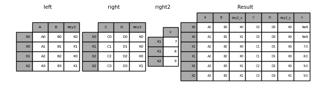
17.2.4 Example 2: Merging with Different Column Names

What if the key columns have different names in each DataFrame? Use the left_on and right_on parameters to specify which columns to match.

# Example: Suppose the external dataset uses 'ID' instead of 'FellowshipID'
# Let's create a version with a different column name to demonstrate
df_external_renamed = df_external.rename(columns={'FellowshipID': 'ID'})

print("External dataset columns after renaming:")
print(list(df_external_renamed.columns))
print()

# Now merge using left_on and right_on
df_merged_diff = pd.merge(
    df_existing, 
    df_external_renamed,
    left_on='FellowshipID',   # Column name in left DataFrame
    right_on='ID'              # Column name in right DataFrame
)

print(f"Merged dataset shape: {df_merged_diff.shape}")
print(f"Merged columns: {list(df_merged_diff.columns)}\n")

df_merged_diff.head()

Important observations:

• Notice that both key columns (FellowshipID and ID) appear in the result
• They contain identical values (the matched keys)
• You can drop one of them after merging: df_merged_diff.drop('ID', axis=1)

Common use case: Merging data from different sources where column naming conventions differ (e.g., customer_id vs cust_id, date vs timestamp).

17.2.5 Example 3: Merging on Multiple Columns

Sometimes you need to match rows based on multiple columns together (composite keys). This is common when a single column isn’t unique.

# Example: Merge on both Name AND Race to ensure exact matches
df_multi_key = pd.merge(
    df_existing, 
    df_external,
    on=['Name', 'Race']  # Both columns must match
)

print(f"Merged on multiple keys: {df_multi_key.shape}")
print("\nMerging on multiple columns ensures rows match on ALL specified keys\n")

df_multi_key.head()

Real-world examples of composite keys:

• Sales transactions: Match on both Store_ID AND Date (same store can have sales on different dates)
• Student grades: Match on Student_ID AND Course_ID (same student takes multiple courses)
• Time series data: Match on Location AND Timestamp (multiple locations measured over time)

Syntax variations:

# Using on= (when column names are the same)
pd.merge(df1, df2, on=['col1', 'col2'])

# Using left_on= and right_on= (when column names differ)
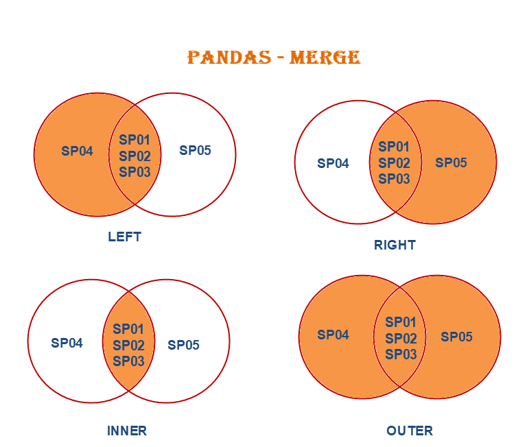
pd.merge(df1, df2, left_on=['id', 'date'], right_on=['ID', 'timestamp'])

17.2.6 Understanding Join Types: The how Parameter

By default, merge() performs an inner join, which keeps only rows where the key exists in both DataFrames. However, you can control this behavior using the how parameter.

The Four Join Types:

Join Type	how=	Keeps Rows From	Use Case
Inner	'inner'	Both (intersection)	Only matching records
Left	'left'	All from left + matches from right	Keep all primary data
Right	'right'	All from right + matches from left	Keep all secondary data
Outer	'outer'	Both (union)	Keep everything

Let’s explore each type with examples.

17.2.6.1 Inner Join (Default): Only Matching Rows

An inner join returns only the rows where the key exists in both DataFrames. This is the default behavior.

# Inner join - explicitly specified (same as default)
df_inner = pd.merge(df_existing, df_external, how='inner')

print(f"Inner join result: {df_inner.shape}")
print("Only rows with matching keys in BOTH datasets are kept\n")

df_inner.head()

Inner join result: (2, 4)
Only rows with matching keys in BOTH datasets are kept

	FellowshipID	FirstName	Skills	Age
0	1001	Frodo	Hiding	50
1	1002	Samwise	Gardening	39

When to use inner join:

Use inner join when you need complete information from both datasets for your analysis.

Real-world examples:

1. Analyzing vaccination impact on COVID infection rates

   • Dataset 1: COVID infection rates by country
   • Dataset 2: Vaccination counts by country
   • Why inner join? You can’t analyze the relationship unless you have BOTH metrics for a country. Countries missing either value can’t contribute to the analysis.

2. Customer purchase analysis

   • Dataset 1: Customer demographics
   • Dataset 2: Purchase transactions
   • Why inner join? To analyze how demographics relate to purchases, you need both demographic info AND purchase history.

3. A/B testing results

   • Dataset 1: User group assignments (control/treatment)
   • Dataset 2: Conversion outcomes
   • Why inner join? Only users with both group assignment AND outcome data can be included in the test analysis.

17.2.6.2 Left Join: Keep All Left DataFrame Rows

A left join returns all rows from the left DataFrame and matching rows from the right DataFrame. Non-matching rows from the right will have NaN values.

# Left join - keep all rows from left (existing) dataset
df_left = pd.merge(df_existing, df_external, how='left')

print(f"Left DataFrame shape: {df_existing.shape}")
print(f"Right DataFrame shape: {df_external.shape}")
print(f"Left join result: {df_left.shape}")
print("\nAll rows from LEFT dataset are kept, even if no match in RIGHT\n")

# Show rows with missing values from the right dataset
missing_count = df_left.isnull().any(axis=1).sum()
print(f"Rows with NaN values (no match in right dataset): {missing_count}\n")

df_left.head(10)

Left DataFrame shape: (4, 3)
Right DataFrame shape: (5, 3)
Left join result: (4, 4)

All rows from LEFT dataset are kept, even if no match in RIGHT

Rows with NaN values (no match in right dataset): 2

	FellowshipID	FirstName	Skills	Age
0	1001	Frodo	Hiding	50.0
1	1002	Samwise	Gardening	39.0
2	1003	Gandalf	Spells	NaN
3	1004	Pippin	Fireworks	NaN

When to use left join:

Use left join when the left dataset contains your primary data that must be retained, while the right dataset provides supplementary information that may be missing for some records.

Real-world examples:

1. COVID infection rates + government effectiveness scores

   • Left: COVID infection rates (critical, hard to impute)
   • Right: Government effectiveness scores (can be estimated from GDP, crime rate, etc.)
   • Why left join? Keep all countries with infection rate data. Missing government scores can be imputed later using correlated variables.

2. Customer demographics + credit card spending

   • Left: Customer demographics (all customers)
   • Right: Credit card transactions (only customers who made purchases)
   • Why left join? Keep all customers, even those with no purchases. Missing spend can be filled with 0 (indicating no transactions).

3. Employee records + performance reviews

   • Left: All employee records
   • Right: Recent performance reviews (not all employees reviewed yet)
   • Why left join? Maintain complete employee roster. Missing reviews can be handled separately (e.g., Pending status).

Key principle: Use left join when you can’t afford to lose the left dataset’s records, and missing right-side values can be reasonably handled (imputed, filled with defaults, or marked as missing).

17.2.6.3 Right Join: Keep All Right DataFrame Rows

A right join is the mirror image of a left join—it returns all rows from the right DataFrame and matching rows from the left DataFrame.

# Right join - keep all rows from right (external) dataset  
df_right = pd.merge(df_existing, df_external, how='right')

print(f"Left DataFrame shape: {df_existing.shape}")
print(f"Right DataFrame shape: {df_external.shape}")
print(f"Right join result: {df_right.shape}")
print("\nAll rows from RIGHT dataset are kept, even if no match in LEFT\n")

df_right.head()

Left DataFrame shape: (4, 3)
Right DataFrame shape: (5, 3)
Right join result: (5, 4)

All rows from RIGHT dataset are kept, even if no match in LEFT

	FellowshipID	FirstName	Skills	Age
0	1001	Frodo	Hiding	50
1	1002	Samwise	Gardening	39
2	1006	Legolas	NaN	2931
3	1007	Elrond	NaN	6520
4	1008	Barromir	NaN	51

When to use right join:

Right join serves the same purpose as left join, just with the DataFrames swapped. In practice:

• Most analysts prefer left join because it’s more intuitive (reads left-to-right)
• Right join is rarely used - you can always swap the DataFrames and use left join instead

Example equivalence:

# These produce the same result:
df_right = pd.merge(df_A, df_B, how='right')  # Right join
df_left = pd.merge(df_B, df_A, how='left')    # Equivalent left join

When you might see right join:

• Legacy code or specific coding style preferences
• SQL background where RIGHT JOIN might be more familiar
• Method chaining where the order is determined by workflow

Best practice: Stick with left join and arrange your DataFrames accordingly—it makes code more readable and maintainable.

17.2.6.4 Outer Join: Keep All Rows from Both DataFrames

An outer join (also called a full outer join) returns all rows from both DataFrames, with NaN values where matches don’t exist. This is the most inclusive join type—no data is lost.

# Outer join - keep all rows from BOTH datasets
df_outer = pd.merge(df_existing, df_external, how='outer')

print(f"Left DataFrame shape: {df_existing.shape}")
print(f"Right DataFrame shape: {df_external.shape}")
print(f"Outer join result: {df_outer.shape}")
print("\nAll rows from BOTH datasets are kept, with NaN for non-matches\n")

# Check for missing values
print("Missing values per column:")
print(df_outer.isnull().sum())
print()

df_outer

Left DataFrame shape: (4, 3)
Right DataFrame shape: (5, 3)
Outer join result: (7, 4)

All rows from BOTH datasets are kept, with NaN for non-matches

Missing values per column:
FellowshipID    0
FirstName       0
Skills          3
Age             2
dtype: int64

	FellowshipID	FirstName	Skills	Age
0	1001	Frodo	Hiding	50.0
1	1002	Samwise	Gardening	39.0
2	1003	Gandalf	Spells	NaN
3	1004	Pippin	Fireworks	NaN
4	1006	Legolas	NaN	2931.0
5	1007	Elrond	NaN	6520.0
6	1008	Barromir	NaN	51.0

When to use outer join:

Use outer join when you cannot afford to lose any data from either dataset, even if it means having incomplete records.

Real-world examples:

1. Course surveys from multiple time points

   • Dataset 1: Mid-semester survey responses
   • Dataset 2: End-of-semester survey responses
   • Why outer join? Students who responded to either survey provide valuable feedback. Keep all responses, even from students who only completed one survey. Analyze response patterns and sentiment across all participants.

2. Multi-source customer data integration

   • Dataset 1: Online purchase records
   • Dataset 2: In-store purchase records
   • Why outer join? Customers may shop through one channel only. Keep all customers to understand total customer base and channel preferences.

3. Scientific study with partial data

   • Dataset 1: Lab test results
   • Dataset 2: Clinical observations
   • Why outer join? Some subjects may have only lab results or only clinical observations due to scheduling, dropouts, or data collection issues. Keep all subjects to maximize sample size and identify patterns in data availability.

4. Data quality auditing

   • Dataset 1: Expected records (should exist)
   • Dataset 2: Actual records (what we have)
   • Why outer join? Identify both missing expected records (in left but not right) and unexpected extra records (in right but not left) for data quality assessment.

Key principle: Use outer join when completeness trumps having matched pairs, and you’ll handle missing values appropriately in subsequent analysis.

17.3 Method 2: Joining with join()

While merge() combines DataFrames based on column values, the join() method combines them based on their indices. This is particularly useful when your DataFrames are already indexed by a meaningful key (like customer ID, timestamp, etc.).

17.3.1 Key Difference: merge() vs join()

Aspect	merge()	join()
Joins on	Column values	Index values
Default join	Inner	Left
Syntax	More explicit	More concise
Use when	Keys are in columns	Keys are in index

17.3.2 Important: Handling Overlapping Columns

Unlike merge(), join() requires you to specify suffixes for overlapping column names (it has no default). This is done with the lsuffix and rsuffix parameters.

Let’s see what happens without suffixes:

The code above will raise an error because both DataFrames have overlapping column names, and join() doesn’t know how to handle them without suffixes.

Let’s fix this by adding suffixes:

# Join with suffixes to handle overlapping column names
df_joined = df_existing.join(
    df_external, 
    lsuffix='_existing',  # Suffix for left DataFrame columns
    rsuffix='_external'    # Suffix for right DataFrame columns
)

print(f"Joined dataset shape: {df_joined.shape}")
print(f"\nColumns with suffixes:")
print([col for col in df_joined.columns if '_existing' in col or '_external' in col])
print()

df_joined.head()

Joined dataset shape: (4, 6)

Columns with suffixes:
['FellowshipID_existing', 'FirstName_existing', 'FellowshipID_external', 'FirstName_external']

	FellowshipID_existing	FirstName_existing	Skills	FellowshipID_external	FirstName_external	Age
0	1001	Frodo	Hiding	1001	Frodo	50
1	1002	Samwise	Gardening	1002	Samwise	39
2	1003	Gandalf	Spells	1006	Legolas	2931
3	1004	Pippin	Fireworks	1007	Elrond	6520

Key Observations:

1. Default behavior: join() performs a left join by default (keeps all rows from the left DataFrame)
2. Index-based: Rows are matched using the DataFrame indices (0, 1, 2, …)
3. Suffixes required: Overlapping column names get the specified suffixes

This works, but notice we’re joining on the default integer index (0, 1, 2, …), which may not be meaningful. Let’s make this more useful by setting a proper index.

17.3.3 Setting a Meaningful Index for Joining

For join() to be truly useful, we should set a meaningful column as the index (like FellowshipID). This way, rows are matched based on actual business logic, not arbitrary row numbers.

# Set 'FellowshipID' as the index for both DataFrames
df_existing_indexed = df_existing.set_index('FellowshipID')
df_external_indexed = df_external.set_index('FellowshipID')

print("Left DataFrame (indexed by Fellowship ID):")
print(df_existing_indexed.head())
print("\nRight DataFrame (indexed by FellowshipID):")
print(df_external_indexed.head())

Left DataFrame (indexed by Fellowship ID):
             FirstName     Skills
FellowshipID                     
1001             Frodo     Hiding
1002           Samwise  Gardening
1003           Gandalf     Spells
1004            Pippin  Fireworks

Right DataFrame (indexed by FellowshipID):
             FirstName   Age
FellowshipID                
1001             Frodo    50
1002           Samwise    39
1006           Legolas  2931
1007            Elrond  6520
1008          Barromir    51

# Now join using the FellowshipID index
df_joined_indexed = df_existing_indexed.join(
    df_external_indexed, 
    lsuffix='_existing',
    rsuffix='_external'
)

print(f"Joined dataset shape: {df_joined_indexed.shape}")
print(f"\nIndex name: {df_joined_indexed.index.name}")
print("\nNow rows are matched by FellowshipID, not arbitrary row numbers!\n")

df_joined_indexed

Joined dataset shape: (4, 4)

Index name: FellowshipID

Now rows are matched by FellowshipID, not arbitrary row numbers!

	FirstName_existing	Skills	FirstName_external	Age
FellowshipID
1001	Frodo	Hiding	Frodo	50.0
1002	Samwise	Gardening	Samwise	39.0
1003	Gandalf	Spells	NaN	NaN
1004	Pippin	Fireworks	NaN	NaN

Perfect! Now the join is meaningful:

• Rows are matched by FellowshipID (a business key)
• All rows from the left DataFrame are kept (default left join)
• NaN values appear where FellowshipID doesn’t exist in the right DataFrame
• The index preserves the key for easy lookup

17.3.4 Changing Join Type in join()

Just like merge(), you can specify the join type using the how parameter:

# Examples of different join types with join()
print("Inner join:")
print(df_existing_indexed.join(df_external_indexed, how='inner', lsuffix='_L', rsuffix='_R').shape)

print("\nOuter join:")
print(df_existing_indexed.join(df_external_indexed, how='outer', lsuffix='_L', rsuffix='_R').shape)

print("\nRight join:")
print(df_existing_indexed.join(df_external_indexed, how='right', lsuffix='_L', rsuffix='_R').shape)

Inner join:
(2, 4)

Outer join:
(7, 4)

Right join:
(5, 4)

17.4 Method 3: Concatenating with concat()

While merge() and join() combine DataFrames by matching keys or indices, concat() simply stacks DataFrames together either vertically (one on top of another) or horizontally (side by side). Think of it as physically gluing DataFrames together.

17.4.1 The Two Directions: axis Parameter

axis=	Direction	Effect	Use Case
0 (default)	Vertical	Rows on top of rows	Combining data from multiple time periods
1	Horizontal	Columns side by side	Adding new features/attributes

17.4.2 Concatenating Along Rows (Vertical Stacking)

The default behavior (axis=0) stacks DataFrames vertically—adding more rows.

17.4.2.1 Simple Example with Fellowship Data

Let’s start with a simple example using our LOTR datasets to understand the basics:

# Split our LOTR data into two groups to demonstrate concatenation
lotr_df1 = df_existing.head(5)  # First 5 fellowship members
lotr_df2 = df_existing.tail(4)  # Last 4 fellowship members

print("First group:")
print(lotr_df1)
print("\nSecond group:")
print(lotr_df2)

# Concatenate vertically (default: axis=0) - stack rows
lotr_combined = pd.concat([lotr_df1, lotr_df2])

print(f"First group: {lotr_df1.shape}")
print(f"Second group: {lotr_df2.shape}")
print(f"Combined: {lotr_combined.shape}")
print("\nRows are simply stacked on top of each other:\n")

lotr_combined

Key points about vertical concatenation:

• Rows are simply stacked (group 1 rows, then group 2 rows)
• Index values may be duplicated (notice indices 0-4 appear, then 5-8)
• All columns from both DataFrames are kept
• No key matching occurs—just physical stacking

Use ignore_index=True to create a new sequential index:

# Reset index to create sequential numbering
lotr_combined_reset = pd.concat([lotr_df1, lotr_df2], ignore_index=True)

print("With ignore_index=True, we get a clean sequential index:\n")
lotr_combined_reset

17.4.2.2 Real-World Example: Combining Continental Data

Now let’s see a practical real-world use case: combining GDP and life expectancy data that’s been split across multiple files by continent. This is a common scenario when data is stored in separate files for organizational purposes.

data_asia = pd.read_csv('./Datasets/gdp_lifeExpec_Asia.csv')
data_europe = pd.read_csv('./Datasets/gdp_lifeExpec_Europe.csv')
data_africa = pd.read_csv('./Datasets/gdp_lifeExpec_Africa.csv')
data_oceania = pd.read_csv('./Datasets/gdp_lifeExpec_Oceania.csv')
data_americas = pd.read_csv('./Datasets/gdp_lifeExpec_Americas.csv')

#Appending all the data files, i.e., stacking them on top of each other
data_all_continents = pd.concat([data_asia,data_europe,data_africa,data_oceania,data_americas],keys = ['Asia','Europe','Africa','Oceania','Americas'])
data_all_continents

		country	year	lifeExp	pop	gdpPercap
Asia	0	Afghanistan	1952	28.801	8425333	779.445314
	1	Afghanistan	1957	30.332	9240934	820.853030
	2	Afghanistan	1962	31.997	10267083	853.100710
	3	Afghanistan	1967	34.020	11537966	836.197138
	4	Afghanistan	1972	36.088	13079460	739.981106
...	...	...	...	...	...	...
Americas	295	Venezuela	1987	70.190	17910182	9883.584648
	296	Venezuela	1992	71.150	20265563	10733.926310
	297	Venezuela	1997	72.146	22374398	10165.495180
	298	Venezuela	2002	72.766	24287670	8605.047831
	299	Venezuela	2007	73.747	26084662	11415.805690

1704 rows × 5 columns

Let’s have the continent as a column as we need to use that in the visualization.

data_all_continents.reset_index(inplace = True)
data_all_continents.head()

	level_0	level_1	country	year	lifeExp	pop	gdpPercap
0	Asia	0	Afghanistan	1952	28.801	8425333	779.445314
1	Asia	1	Afghanistan	1957	30.332	9240934	820.853030
2	Asia	2	Afghanistan	1962	31.997	10267083	853.100710
3	Asia	3	Afghanistan	1967	34.020	11537966	836.197138
4	Asia	4	Afghanistan	1972	36.088	13079460	739.981106

data_all_continents.drop(columns = 'level_1',inplace = True)
data_all_continents.rename(columns = {'level_0':'continent'},inplace = True)
data_all_continents.head()

	continent	country	year	lifeExp	pop	gdpPercap
0	Asia	Afghanistan	1952	28.801	8425333	779.445314
1	Asia	Afghanistan	1957	30.332	9240934	820.853030
2	Asia	Afghanistan	1962	31.997	10267083	853.100710
3	Asia	Afghanistan	1967	34.020	11537966	836.197138
4	Asia	Afghanistan	1972	36.088	13079460	739.981106

#change of life expectancy over time for different continents
a = sns.FacetGrid(data_all_continents,col = 'continent',col_wrap = 3,height = 4.5,aspect = 1)#height = 3,aspect = 0.8)
a.map(sns.lineplot,'year','lifeExp')
a.add_legend();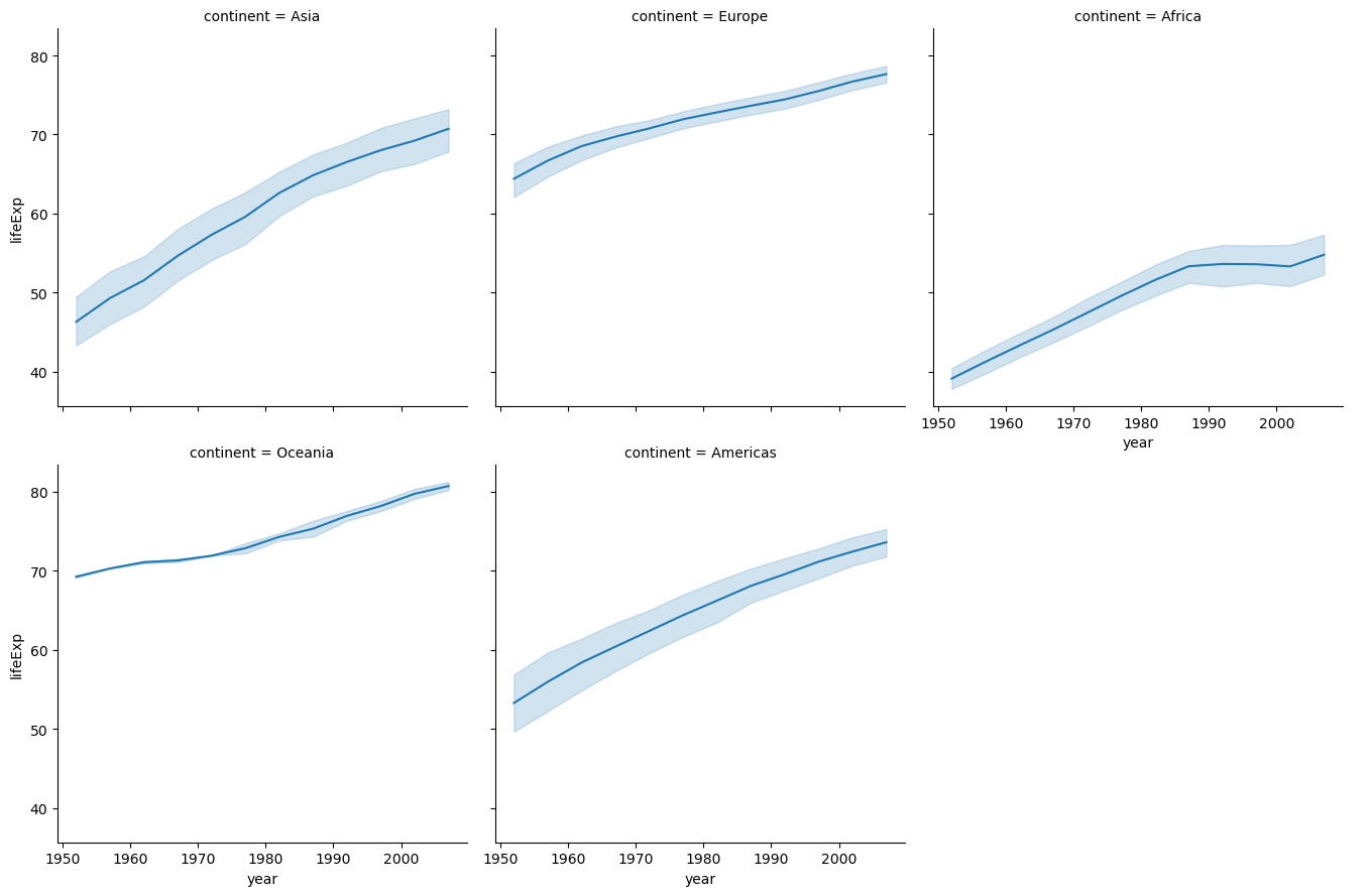

In the above example, datasets were appended (or stacked on top of each other).

Datasets can also be concatenated side-by-side (by providing the argument axis = 1 with the concat() function) as we saw with the merge function.

17.4.3 Horizontal Concatenation (Combining Columns)

Setting axis=1 combines DataFrames side-by-side by aligning their indices.

# Concatenate horizontally (axis=1) - combine columns
result = pd.concat([df_existing, df_external], axis=1)
result

	FellowshipID	FirstName	Skills	FellowshipID	FirstName	Age
0	1001.0	Frodo	Hiding	1001	Frodo	50
1	1002.0	Samwise	Gardening	1002	Samwise	39
2	1003.0	Gandalf	Spells	1006	Legolas	2931
3	1004.0	Pippin	Fireworks	1007	Elrond	6520
4	NaN	NaN	NaN	1008	Barromir	51

Notice:

• DataFrames are placed side-by-side
• Index values are used for alignment (matching FellowshipIDs are aligned)
• Non-matching indices result in NaN values
• This is similar to an outer join on the index

When to use horizontal concat:

• Adding new features/columns to existing data
• Combining results from different analyses on the same observations
• Building feature matrices for machine learning (each DataFrame contains different feature sets)

17.4.3.1 Handling Duplicate Column Names

When concatenating horizontally with duplicate column names, pandas keeps both columns:

# See column names when both DataFrames have 'Name'
result.columns

Index(['FellowshipID', 'FirstName', 'Skills', 'FellowshipID', 'FirstName',
       'Age'],
      dtype='object')

Both Name columns are kept, which can be confusing. You can use the keys parameter to create hierarchical column names:

# Use keys to label which DataFrame each column came from
result_labeled = pd.concat([df_existing, df_external], axis=1, keys=['Fellowship', 'Extended'])
result_labeled

	Fellowship			Extended
	FellowshipID	FirstName	Skills	FellowshipID	FirstName	Age
0	1001.0	Frodo	Hiding	1001	Frodo	50
1	1002.0	Samwise	Gardening	1002	Samwise	39
2	1003.0	Gandalf	Spells	1006	Legolas	2931
3	1004.0	Pippin	Fireworks	1007	Elrond	6520
4	NaN	NaN	NaN	1008	Barromir	51

Now you can clearly see which DataFrame each column came from. This creates a MultiIndex for columns (we’ll cover this in detail in future chapters).

17.5 Summary: Choosing the Right Method

Now that we’ve covered all three methods for combining DataFrames, here’s how to choose:

Method	Best For	Key Feature	Common Pitfall
merge()	Combining on shared column(s)	Flexible join types (inner/left/right/outer)	Forgetting to specify join type (defaults to inner)
join()	Combining on index values	Quick syntax for index-based joins	Index must be set up properly beforehand
concat()	Stacking DataFrames with same structure	Simple vertical/horizontal stacking	Doesn’t match on keys (just stacks/aligns)

17.5.1 Decision Tree:

1. Do you need to match rows based on values in columns?

   • Yes → Use merge() (specify join type and on= parameter)

2. Do you need to match rows based on index values?

   • Yes → Use join() (ensure indices are meaningful)

3. Do you just need to stack DataFrames?

   • Vertically (add more rows) → Use concat(axis=0)
   • Horizontally (add more columns) → Use concat(axis=1) (aligns on index)

17.6 Handling Missing Values After Combining Datasets

When you combine datasets using merge(), join(), or concat(), you often introduce missing values (NaN) for unmatched entries. Understanding why these appear and how to handle them is crucial for maintaining data quality.

17.6.1 Why Missing Values Occur

Missing values appear for different reasons depending on the join type:

Join Type	When NaN Appears	Example
Left Join	Right DataFrame has no match for left keys	Customer exists but has no purchases → purchase columns = NaN
Right Join	Left DataFrame has no match for right keys	Purchase exists but customer deleted → customer columns = NaN
Outer Join	Either DataFrame has no match	Missing data from both sides
concat (axis=1)	Indices don’t align	Different row indices → NaN where no alignment

Inner joins never produce NaN from the join operation itself (only matched rows are kept).

17.6.2 Strategies for Handling Missing Values

The right strategy depends on why the data is missing and what you’re analyzing.

17.6.2.1 Strategy 1: Keep the Missing Values

When to use: Missing values are meaningful and represent absence of something.

Example: Customer purchase analysis with left join

# All customers + their purchases (if any)
df_customer_purchases = customers.merge(purchases, on='CustomerID', how='left')

Interpretation:

• NaN in purchase columns = Customer hasn’t made a purchase yet
• This is informative - these customers might be new or inactive
• Analysis: What percentage of customers have never purchased? requires keeping NaN

Action: Keep NaN and analyze it as a category (e.g., df['Purchase'].isna().sum())

17.6.2.2 Strategy 2: Fill with Default Values

When to use: Missing values should be interpreted as zero or a default state.

Example: Sales data where no transaction = zero sales

# Fill missing sales with 0
df_merged['TotalSales'] = df_merged['TotalSales'].fillna(0)
df_merged['TransactionCount'] = df_merged['TransactionCount'].fillna(0)

Common fill values:

• 0 - for counts, amounts, quantities
• 'None' or 'Unknown' - for categorical data
• False - for boolean flags
• Mean/median - for numerical features (use with caution!)

Caution: Only fill when you’re certain what the missing value means.

17.6.2.3 Strategy 3: Drop Rows with Missing Values

When to use: Analysis requires complete information from both datasets.

Example: Analyzing relationship between two variables (need both)

# Drop rows where either GDP or Population is missing
df_complete = df_merged.dropna(subset=['GDP', 'Population'])

Options:

• dropna() - drop rows with any NaN
• dropna(subset=['col1', 'col2']) - drop only if specific columns have NaN
• dropna(thresh=5) - drop only if fewer than 5 non-NaN values

Caution: You’re losing data! Document how many rows were dropped and why.

17.6.2.4 Strategy 4: Use a Different Join Type

When to use: You’re getting NaN because you used the wrong join type!

Example: Used outer join but only need matching rows

# Wrong: Creates many NaN values
df_outer = pd.merge(df1, df2, how='outer')  # 1000 rows, 50% NaN

# Better: Use inner join to keep only complete matches
df_inner = pd.merge(df1, df2, how='inner')  # 600 rows, 0% NaN

Before handling missing values, ask: 1. Did I use the right join type for my analysis question? 2. Should I actually be using inner join instead of left/outer? 3. Are the missing values telling me about data quality issues?

17.6.3 Practical Example: Handling Missing Values

Let’s see these strategies in action with our fellowship data:

# Create an outer join to see missing values
df_outer_example = pd.merge(df_existing, df_external, how='outer')

print("Outer join result:")
print(f"Total rows: {len(df_outer_example)}")
print(f"\nMissing values per column:")
print(df_outer_example.isnull().sum())
print(f"\nRows with ANY missing value: {df_outer_example.isnull().any(axis=1).sum()}")

df_outer_example

Now let’s apply different strategies:

# Strategy 1: Identify WHERE the missing values are
print("Rows with missing 'Race' (from left dataset):")
print(df_outer_example[df_outer_example['Race'].isna()][['Name', 'Race', 'Birthplace']])
print()

print("Rows with missing 'Birthplace' (from right dataset):")
print(df_outer_example[df_outer_example['Birthplace'].isna()][['Name', 'Race', 'Birthplace']])

# Strategy 2: Drop incomplete rows (for complete-case analysis)
df_complete = df_outer_example.dropna()

print(f"Original rows: {len(df_outer_example)}")
print(f"Complete rows: {len(df_complete)}")
print(f"Rows dropped: {len(df_outer_example) - len(df_complete)}")
print()
df_complete

# Strategy 3: Fill with meaningful defaults
df_filled = df_outer_example.copy()
df_filled['Birthplace'] = df_filled['Birthplace'].fillna('Unknown')

print("After filling missing 'Birthplace' with 'Unknown':")
print(df_filled[['Name', 'Birthplace']])
print(f"\nMissing 'Birthplace' values: {df_filled['Birthplace'].isna().sum()}")

17.6.4 Best Practices for Missing Value Handling

1. Investigate First

# Always check WHERE and WHY values are missing
df.isnull().sum()  # Count per column
df[df['column'].isna()]  # See the actual rows

2. Document Your Decisions

# Good: Document what you did and why
# Filled missing GDP with 0 because these are countries with no economic data reported
df['GDP'] = df['GDP'].fillna(0)

# Also good: Create a flag for missing values before filling
df['GDP_was_missing'] = df['GDP'].isna()
df['GDP'] = df['GDP'].fillna(df['GDP'].median())

3. Consider the Impact

• Dropping rows: Reduces sample size, may introduce bias
• Filling with defaults: May distort statistics (mean, correlations)
• Keeping NaN: Requires careful handling in analysis/visualization

4. Choose Join Type Carefully

The best way to handle missing values is often to prevent them by using the right join type for your analysis question!

Remember: Missing values after combining datasets are expected and normal. The key is understanding what they mean and handling them appropriately for your specific analysis goals.

17.7 Independent Study

17.7.1 Merging GDP per capita and population datasets

In this independent study on data reshaping, we have provided two datasets:
- gdp_per_capita_data
- population_data

This exercise builds on the results from the previous section.

Task:
Merge gdp_per_capita_data with population_data to combine each country’s population and GDP per capita into a single DataFrame.
Finally, print the first two rows of the merged DataFrame.

Assume that:

1. We want to keep the GDP per capita of all countries in the merged dataset, even if their population in unavailable in the population dataset. For countries whose population in unavailable, their Population column will show NA.

2. We want to discard an observation of a country if its GDP per capita is unavailable.

17.7.1.1

For how many countries in gdp_per_capita_data does the population seem to be unavailable in population_data? Note that you don’t need to clean country names any further than cleaned by the functions provided.

Print the observations of gdp_per_capita_data with missing Population.

17.7.2 Merging datasets with similar values in the key column

We suspect that population of more countries may be available in population_data. However, due to unclean country names, the observations could not merge. For example, the country Guinea Bissau is mentioned as GuineaBissau in gdp_per_capita_data and Guinea-Bissau in population_data. To resolve this issue, we’ll use a different approach to merge datasts. We’ll merge the population of a country to an observation in the GDP per capita dataset, whose name in population_data is the most similar to the name of the country in gdp_per_capita_data.

17.7.2.1

Proceed as follows:

1. For each country in gdp_per_capita_data, find the country with the most similar name in population_data, based on the similarity score. Use the lambda function provided below to compute the similarity score between two strings (The higher the score, the more similar are the strings. The similarity score is \(1.0\) if two strings are exactly the same).

2. Merge the population of the most similar country to the country in gdp_per_capita_data. The merged dataset must include 5 columns - the country name as it appears in gdp_per_capita_data, the GDP per capita, the country name of the most similar country as it appears in population_data, the population of that country, and the similarity score between the country names.

3. After creating the merged dataset, print the rows of the dataset that have similarity scores less than 1.

Use the function below to compute the similarity score between the Country names of the two datasets:

from difflib import SequenceMatcher

similar = lambda a,b: SequenceMatcher(None, a, b).ratio()

Note: You may use one for loop only for this particular question. However, it would be perfect if don’t use a for loop

Hint:

1. Define a function that computes the index of the observation having the most similar country name in population_data for an observation in gdp_per_capita_data. The function returns a Series consisting of the most similar country name, its population, and its similarity score (This function can be written with only one line in its body, excluding the return statement and the definition statement. However, you may use as many lines as you wish).

2. Apply the function on the Country column of gdp_per_capita_data. A DataFrame will be obtained.

3. Concatenate the DataFrame obtained in (2) with gdp_per_capita_data with the pandas concat() function.

17.7.2.2

In the dataset obtained in the previous question, for all observations where similarity score is less than 0.8, replace the population with Nan.

Print the observations of the dataset having missing values of population.